For as long as I can remember, I’ve dreamed of creating my own content and contributing something of value back to a community that has taught me so much. My own journey, filled with endless searches for clear and meaningful information, has shown me just how vital the simple act of (clearly) explaining things is. Wins a lot of TIME !
Many articles I’ve read on machine learning can feel a bit rushed, often designed more for search engines than for deep understanding. This is why so many of us have found a home in video content, like the brilliant Statquest with Josh Starmer, the amazing Julia Turc and the one and only Andrej Karpathy. All of them make complex ideas feel intuitive and engaging. Yet, for that knowledge to truly set in, we often need to go deeper, to read something long and exhaustive, like the blog of Chris Olah (One of Anthropic co-founders). The blog post you’re reading now is my effort to create an exhaustive resource, that I really really hope it will bring value to whoever is reading !
I chose Random Forests for this deep dive for a few reasons. The topic itself is a perfect vehicle for exploring a wide range of core machine learning concepts. It’s a subject that frequently came up (for me) in technical interviews. There is a certain elegance to them: their logic is surprisingly intuitive, which means the wisdom behind them can be appreciated by anyone, young and old.
We will build our knowledge from the ground up, starting with the absolute basics and moving all the way to the edge of current research (or at least, the edge as of today, since the field never stops improving). My goal is for the reader to enjoy what I enjoy and see what I see, question by question.
So, before we start anything, we first need to understand the terrain. Where exactly in the vast landscape of machine learning do Random Forests fit? And what is even machine learning in the first place, bro ?
The landscape

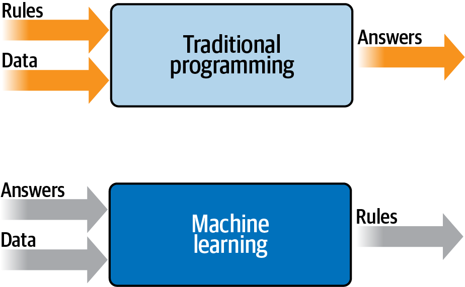
Machine learning is a subfield of computer science that moves away from the paradigm of traditional programming. In a conventional program, a developer writes explicit, step-by-step instructions (the algorithm) that tell the computer exactly how to solve a problem. If you want to filter spam, you might write a rule like:
IF email_subject CONTAINS "free money" THEN mark_as_spam
This approach is brittle and fails as soon as spammers change their tactics (and they do this a lot :D). Machine learning inverts this relationship. Instead of providing the rules, you provide the data (a vast collection of examples of what is and is not spam) and an algorithm that can infer the rules from those examples. It studies all these examples and automatically discovers the patterns in the data, optimizing its approach with each example until it gets really good at telling spam from legitimate emails. This trial-and-refinement process is what we call “learning.”
The output of this learning process is what we call a “model.” We use this term because the result is a simplified, learned representation of the reality found within the data. It is not reality itself, but a useful approximation. This model is the entity that makes the predictions. Crucially, a model is not always a pure mathematical equation. In a linear regression, the model is indeed a specific formula (e.g., Loan_Risk = 0.5*Income - 0.2*Age + ...). However, in other cases, like in Decision Trees (that we will see next) the model is a logical structure: a specific flowchart of if-then rules. The ultimate goal is to produce a model that can generalize,that is, take the rules it has inferred from the historical data and apply them accurately to new, unseen situations.
The methods used to build these models depend entirely on the nature of the problem and the data available. The most common scenario is supervised learning, where the historical data is “labeled” with the correct answers. The algorithm is “supervised” because at every step of its training, it can compare its prediction to the known correct outcome and adjust itself accordingly, to become better at the task. This is the paradigm we will operate in. Within this, if the target we are predicting is a continuous numerical value (like the price of a house, or the weight of a mouse, or your income), the task is called regression. If the target is a discrete category (like ‘spam’ or ‘no spam’), it is called classification. In contrast, there is also unsupervised learning, where the data has no labels. Here, the goal is not to predict a known outcome, but to discover hidden structures within the data itself, such as grouping similar customers into distinct segments.
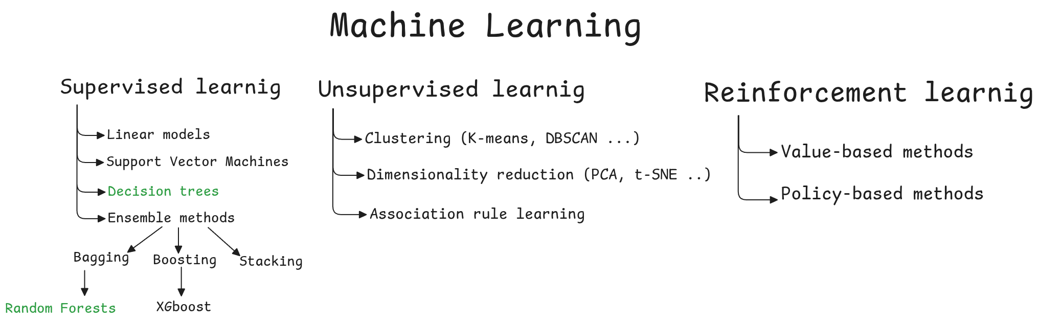
Now, within this supervised learning landscape (like shown in the figure above), under the ensemble methods we can find Random Forests. They’re not the flashiest algorithm (I think that honor probably goes to neural networks), but they’re incredibly popular and reliable. Over 112,000 Kaggle notebooks mention the technique (check here), and it’s been the winning algorithm in numerous machine learning competitions, including major hackathons like the EMC Data Science Global Hackathon (check this paper if you want to dive into the popularity data). Leo Breiman’s 2001 introduction of Random Forests (in this paper) has now been cited over 162,000 times, a testament to how important they are.
But what exactly are they? How do they work? Why do we call them “forests”? Where are the trees?
To answer these questions, we will step by step build the algorithm behind the method, intuitively from scratch and see all the math behind it (without being boring I promise!), the main unit of a Random Forest model is a ‘Decision Tree’, let’s discover what it is, why it works so well on its own, why it’s not sufficient alone, why we need a lot of trees, why they need to be ‘random’ and how do they communicate with each other to make predictions!
Decision trees
The intuition behind this algorithm lies behind a very simple idea: making a sequence of simple decisions to arrive at a complex conclusion.
In order to visualize it well, let’s use a realistic example, something you might actually encounter. Imagine you work for a bank, and your task is to predict whether a new loan applicant is likely to default on their loan. Your historical data might look something like this (The final column, Defaulted, is our target, what we want to predict. The other columns are our features, our helping columns that will lead our prediction):
| Annual Income ($) | Age | Loan Amount ($) | Credit History | Defaulted |
|---|---|---|---|---|
| 35,000 | 24 | 10,000 | Good | No |
| 75,000 | 45 | 50,000 | Good | No |
| 28,000 | 29 | 15,000 | Poor | Yes |
| 110,000 | 52 | 20,000 | Excellent | No |
| 42,000 | 31 | 30,000 | Poor | Yes |
One way to think about this is to simply start asking questions. A human analyst might look at this data and instinctively create rules. “It seems like people with a Poor credit history and a high loan amount tend to default.” This is a natural, intuitive way to reason, and it is precisely the logic that a Decision Tree formalizes, we can see in the figure below our thinking clearly, and yes this is the most basic DT ever.
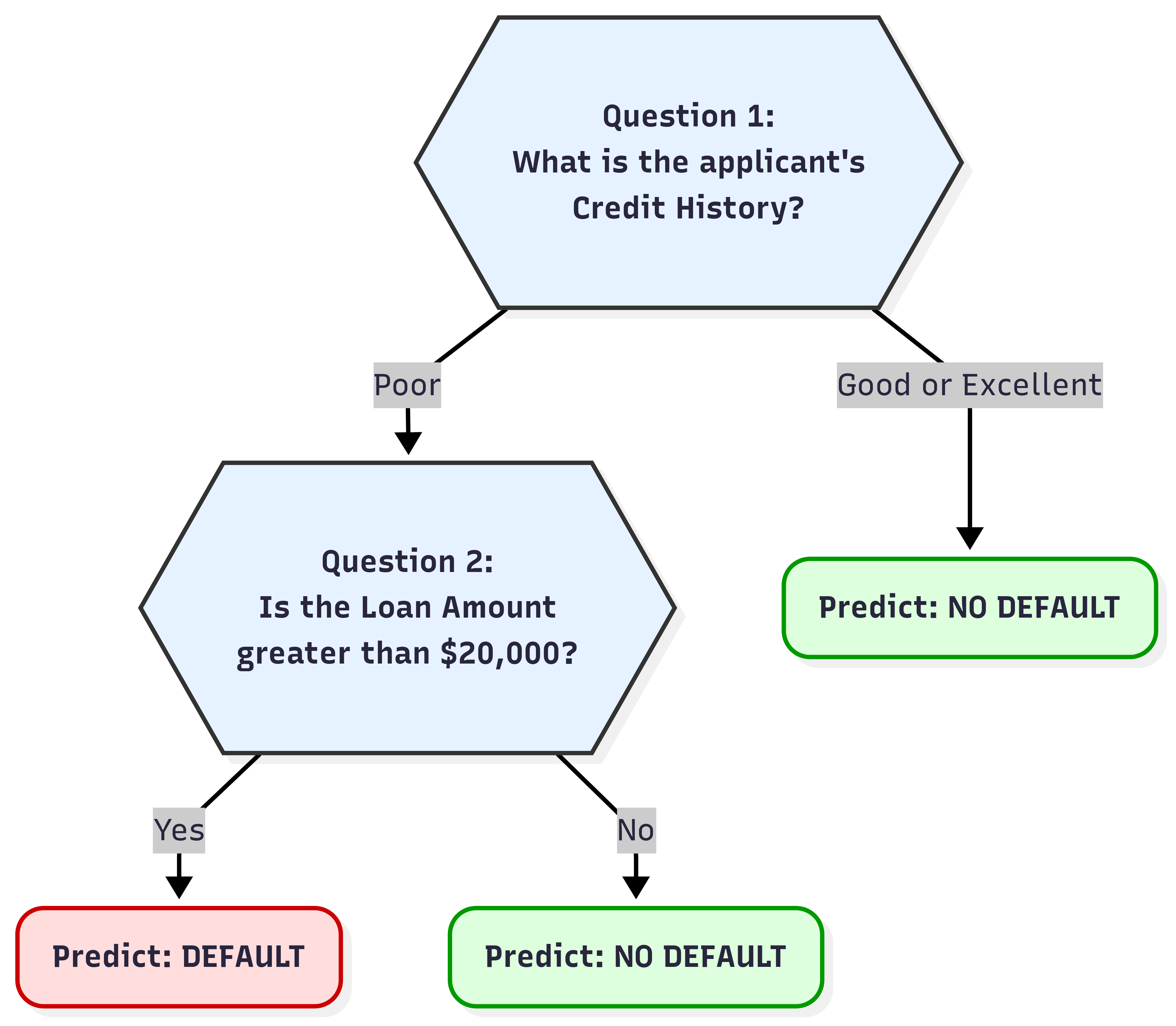
You might be looking at this and thinking it feels incomplete. And you’d be right. After all, we could have asked other questions. What about Is Age > 30? or Is Annual Income < $40,000? Even more importantly, the chaining of these questions could be completely different, we could ask question A before B or add question C or D. The entire structure of our model depends on which questions we ask, and in what order.
Intuitively, the best ‘question’ (or splitting criteria) to ask is the one that splits our data most cleanly. Imagine a split that results in two new groups. In one group, you have applicants who all defaulted. In the other, you have applicants who all did not. This would be a perfect split. Why is this the goal? Because a perfect split creates a perfect rule. If you find such a question (or a chain of questions), you have found a powerful piece of logic for generalization. Any new applicant who fits the criteria (or the chain of criterias) for one of those pure groups can be classified with maximum confidence. It’s the most efficient way to reduce uncertainty.
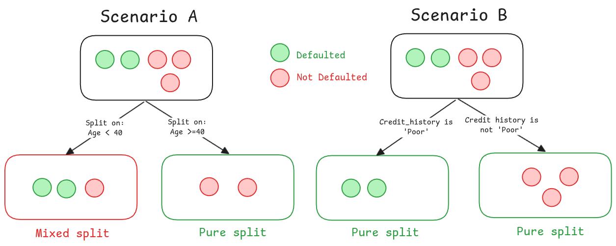
Of course, in the real world, a single perfect split almost never happens. Data is messy. Most of the time, we have to choose between imperfect splits.
So far, we’ve established intuitive ideas, but intuition isn’t something a computer can work with. An algorithm needs a number, a score. We need to mathematically measure the impurity of a group of data.
To do this, let’s throw out the textbook definitions and invent the solution ourselves. We’ll rely on pure statistics and use the concept of probability (which is just a way of quantifying the likelihood of an event happening) to mathematically define this messiness.
Let’s start with a simple game. This game is the entire intuition behind the formula.
- You have a bucket of our 5 loan applicants (3 “No”, 2 “Yes”).
- You reach in and randomly pull one applicant out. You note their label.
- You put them back in (so the odds don’t change), and you randomly pull out a second applicant.
The question that defines our entire metric is this:
What is the probability that both applicants you pulled have the SAME label?
Think about it. If this probability is high, the bucket must be very pure and predictable. If it’s low, the bucket must be a messy, unpredictable mix. This “probability of a random match” is the perfect proxy for purity.
A match can happen in two ways: we pull “No” then “No”, OR we pull “Yes” then “Yes”. The probability of the first event AND the second event both happening is the product of their individual probabilities. Since we can have a “No-No” match OR a “Yes-Yes” match, we add their probabilities together (if you don’t feel at ease with the intuition behind multiplying and adding the probabilties of events read this).
Purity Score = P(No-No match) + P(Yes-Yes match)
Purity Score = (p_No)² + (p_Yes)²
This Σ (pᵢ)² is our Purity Score. But we wanted a score for impurity, where 0 is good (pure) and a high number is bad (messy). We just need to flip it. The opposite of getting a match is getting a mismatch.
Impurity Score = 1 - Purity Score = 1 - Σ (pᵢ)²
And there it is. We have built our needed metric, which (happens that) is officially called the Gini Impurity. It ranges from 0 (perfectly pure) to 0.5 (maximum impurity for a two-class problem), exactly as our intuition would predict.
Now that we have the tool we needed, let’s apply it to our previous example:
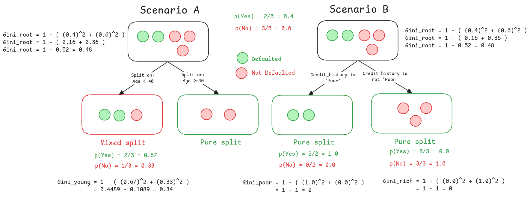
As you can see from the calculations, both scenarios start with the same parent node, which has a Gini Impurity of 0.48, that is a very mixed group.
In Scenario B, the split on Credit History is incredibly effective. It produces two child nodes, and both of them are perfectly pure, each with a Gini Impurity of 0. It has successfully sorted the applicants.
In Scenario A, however, the split on Age is less successful. While it does produce one pure node on the right (Gini = 0), the left node is still a mixed bag of defaulted and non-defaulted applicants, resulting in a Gini Impurity of 0.34. It reduced the messiness, but it didn’t eliminate it.
Intuitively, we know Scenario B is the better choice. But the algorithm needs a final score to compare them directly. It can’t just look at the child nodes individually; it needs a single number that represents the overall “goodness” of the entire split. This is where we introduce Gini Gain.
The idea is simple: the best split is the one that causes the biggest drop in impurity from the parent node to the children.
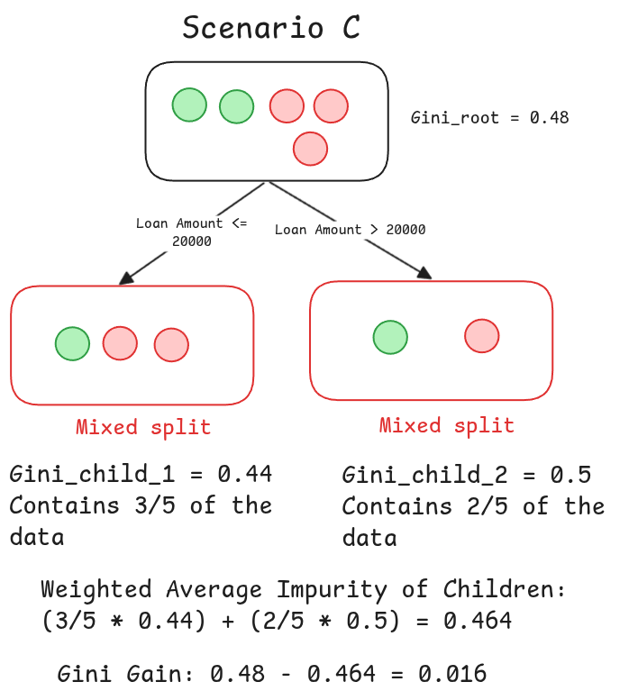
But how do we calculate the total impurity of the children? We can’t just add their Gini scores, because a split that sends 4 people to a pure node and 1 person to a messy one is much better than a split that sends them to two equally messy nodes. The size of the groups matters. So, we calculate a weighted average of the children’s impurity, where the weight is simply the proportion of applicants that ended up in each node.
The formula is just common sense:
Gini Gain = Gini(parent) - [ (weight_child1 * Gini(child1)) + (weight_child2 * Gini(child2)) ]
Now, let’s apply it to our two scenarios and see who wins.
Scenario B: Splitting on Credit History
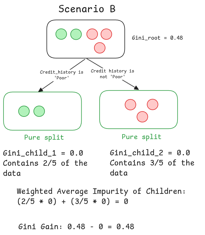
A gain of 0.48! We completely eliminated all the impurity. That makes perfect sense.
Scenario A: Splitting on Age
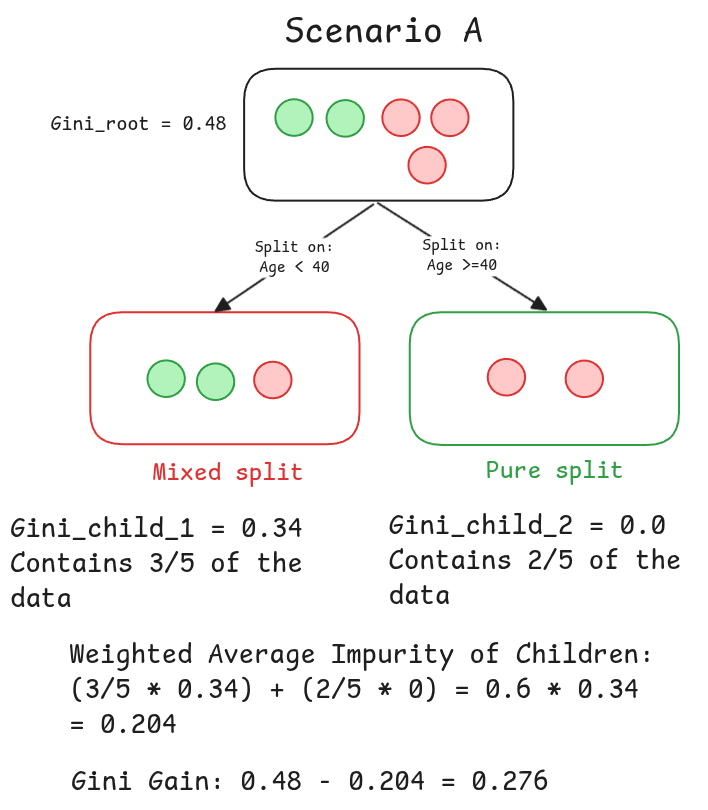
Since 0.48 > 0.276, the algorithm declares the split on Credit History the undisputed winner. This becomes the first, most powerful question in our decision tree.
In fact, we need to do this for all the features and all the values of the features, make a lot of splits and calculate one by one the Gini Gain until we find the best one and make it the root node, in this example we found it directly, but we need to test all the possible values, we perform a brute-force search, so scnearios like that might be added (notice that we found a Gini gain of 0.016, which make this split the worst split, intuitively we can feel it because it resulted in two mixed splits):